Results for Lawson DNA Project

If we review the Lawson Y-DNA 37 Alleles or the Y-DNA 67 Alleles tables, which contain the results of the DNA tests we have had carried out, we can see that we have 6 or more haplogroups associated with the surname of Lawson. Two of these haplogroups, I1 and R1b1, contain the majority of the members of our Project, but given that R1b1 also contains many unrelated haplotypes we might well ask how this can be the case.

If we review the information provided on FamilyTreeDNA's website pertaining to haplogroups and closely examine the Y-DNA Haplogroup Tree (its official name is the Y-Chromosome Phylogenetic Tree and it can be download as a PDF file from the above FamilyTreeDNA website), we can conclude that members of different haplogroups cannot be related to each other within many thousands of years. Since we all share a single surname, how is it possible that we belong to so many different haplogroups and have haplogroups, which are unrelated? Surely our families did not have a significant enough number of non-paternity events or adoptions to provide an explanation? To understand this, we need to look at how our ancestors may have adopted the surname Lawson, which may have led to it belonging to several distinct haplogroups.

The Lawson Surname

The adoption of hereditary surnames in Britain may have originated with the Anglo-French nobility some three or four generations after the Norman Conquest of the British Isles in 1066. Prior to this surnames were not required and most people, who had only a small circle of family and friends, used only a single name. As the population and mobility of peoples increased so did the need for various forms of documentation such as censuses, wills and deeds. To better facilitate identification, the practice of having more than one name became more common. In Western Europe between the twelfth and sixteenth centuries most people had a hereditary surname.

However, some of the Scandinavian Countries, such as Denmark, Sweden and Norway, this development did not take place until the late nineteenth or early twenty century. These countries still made use of what is known as the patronymic system of naming their children.

If we look up the name "Lawson" in the Dictionary of American Family Names (Oxford University Press) to get the history and origin for the surname Lawson we find: -

Scottish and northern English: patronymic from Law (son of Law).
Americanized form of Swedish Larsson or Norwegian/Danish Larssen.

If we review the history and origin of the surname Law we get:

A diminutive or short version of the given name Laurence or Lawrence, from the Roman cognomen Laurentius, meaning "of Laurentum" - a city in ancient Italy.
Possibly derived from the Old English 'hlaw' or 'hyll,' meaning small hill or burial mound; which became "low" in the south, but "law" in the north of England.

Another Dictionary of Names gives the following for Lawrence: -
English: from the Middle English and Old French personal name Lorens, Laurence (Latin Laurentius ‘man from Laurentum’, a place in Italy probably named from its laurels or bay trees). The name was borne by a saint who was martyred at Rome in the 3rd century ad; he enjoyed a considerable cult throughout Europe, with consequent popularity of the personal name (French Laurent, Italian, Spanish Lorenzo, Catalan Llorenç, Portuguese Lourenço, German Laurenz; Polish Wawrzyniec etc.).

Patronymic surnames are derived, either directly or as diminutives, from personal names, followed by a suffix (i.e. s, se, sen, son for boys). Some surnames of this type give clues as to their origin. The suffix of ‘-s’ in Laws is more commonly found in southern England and the Midlands while the ‘-son’ in Lawson is more common in northern England and Lowland Scotland. It was practiced in many areas of Europe for extended periods of time and as an example it only ended in Norway in 1923 when by law it was ordered that each family should have a hereditary last name and only one last name. Here is an example of patronymic naming in Norway prior to this law: -

Father: Lars Olssen
Son: Niels Larssen
Grandson: Hans Nielssen
Great-grandson: Lars Hanssen

Patronymic surnames formed from Laurenti
Latin	English	Greek	Russian	Dutch	Scottish	Swedish/ Norwegian
Laurenti	Lawson Lawrence	Lavrentakis	Lavrentiew	Laarse	MacLaren	Larsson Larssen

There are some important ramifications resulting from this process, other than the obvious. One is that people, today, whose surname is based on a patronymic, may be totally unrelated to other people with the same surname. Picture, if you will, that in 1923, everyone in Norway was mandated to use a surname and most adopted their father's patronymic as a surname. Two brothers, Lars and Niels, now have all their descendants named, respectively, LARSSEN and NIELSSEN — yet these families are closely related. In contrast, two unrelated men named LARS, on opposite sides of Norway, now both have all their descendants surnamed LARSSEN — yet they are not related at all.

As it is easy to see from the example above, between the twelfth and sixteenth centuries, the period when our Lawsons and other Lawsons most likely decided to adopt their hereditary last name from Law, we could end up with a number of families with the same surname, but unrelated and from a number of different haplogroups.

Tools for the Analysis

Alleles Tables

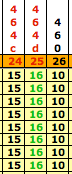
You are probably familiar with the tables that most of the Surname Projects use to group their members and the results for each allele or marker that has been tested by one of the companies that specialize in genetic genealogy such as FamilyTreeDNA (FTDNA). The table usually consists of a column on the left side with the names, kit numbers or some identification for the members. Across the top of the table is the name of the alleles or markers such as DNA Y-chromosome Segment (DYS) -393 or just 393.

In the Lawson DNA Project we have two of these tables, Y-DNA 37 Alleles and Y-DNA 67 Alleles Tables. The 37 Alleles Table includes a column on the right hand side with the names of the three oldest family members of that line, or a short pedigree if it has been submitted to the Project. When FTDNA expanded their test program to include an additional 30 markers, the table became to large to include the short pedigree, so it was dropped from the 67 Alleles Table.

Also incorporated in our tables is a way to contact each member by email. The kit number on the left side of the table, second column, is an active link where you can click and send an email. The third column contains the haplogroup predicted by FTDNA or is the results from tests that the member has had performed. On the right hand side of the table, just before the short pedigree is another active kit number. This one, when clicked on will bring up an expanded pedigree for that member.

To use the tables to analyze the members, we arrange them according to their haplogroups and color-code them. Once this is completed, we find we have two very large haplogroups for the Lawsons and they are haplogroup I1 (yellow group) and R1b1 (blue group). At this point two techniques can be used to break these two large groups into smaller ones. First we use the pedigrees that most of the members have supplied to the project and then in conjunction with the pedigrees we look for clusters, which are a group of haplotypes that have the same number of repeats at one of the markers to help break the large groups into small ones. We have called these clusters “branch markers” and it worked very well with the I1 haplogroup, but not as well with the R1b1 haplogroup. Here are some examples for the I1 group: -

Examples from I1 Group
Group 2 Branch Markers	Group 3 Branch Markers	Possible Branch Markers

Dean McGee’s Y-DNA Utility

Dean McGee has developed his Y-DNA Comparison Utility and made it available on the Internet for free use and it is a very constructive tool for genetic genealogy researchers everywhere. It has facilitated analysis and significantly helped in the assessment of our results and he is due much gratitude for making it available to researchers.

The following is a small example of how to use his utility.

Prepare an Excel file such as the one below.

Examples from R1b1 Group
Excel File Example	Comments
	I have used 12 markers and 16 members in this example

Go to McGee's webpage and open the Y-DNA Comparison Utility and make sure that the heading has “Y-Utility: Y-DNA Comparison Utility, FTDNA Mode”. As you can see there is a Ysearch Mode that you do not want at this time.
Under the “Generate Tables” uncheck all the boxes except “FTDNA order haplotyp comparison” and “Genetic Distance”.
Return to your Excel file and copy the member’s kit numbers and all their markers (all the information in light blue).
Paste the information from your spreadsheet into the area titled “Paste haplotype rows here (without marker headers)” and then hit “Execute”. Your results should look like the tables below.

FTDNA Configuration - DNA Results Comparison

D
Y
S
3
9
3

D
Y
S
3
9
0

D
Y
S
1
9
/
3
9
4

D
Y
S
3
9
1

D
Y
S
3
8
5
a

D
Y
S
3
8
5
b

D
Y
S
4
2
6

D
Y
S
3
8
8

D
Y
S
4
3
9

D
Y
S
3
8
9
-
1

D
Y
S
3
9
2

D
Y
S
3
8
9
-
2

modal

48786

121895

71645

75975

119505

107400

118697

80588

44728

80643

63077

69475

62926

108238

66787

81011

Distance from reference:

Zero

One

Two

Three+

We will not analyze this tables; all that is being done here is demonstrating one of the tools that can be used.

The first table, "DNA Results Comparison," is much the same as our Y-DNA 37 and 67 Charts. It does have one row that is new and is the called “modal”. McGee’s utility calculates this for us and here is how it is done for this chart of 12 members. Look at DYS393, there are 14 members with repeats of 13, one member with 12 and one with 14. Therefore the modal value for this DYS393 is 13. As you can see, the modal value is not the mean or average or the median value, but is just the number that appears most frequently in the list. In the second column, DYS390, 24 appears 12 times and no other number is close, so the modal value for DYS390 is 24.

The utility then tallies up each member’s genetic distance from the modal and color codes each marker that is different from the modal. No color means that marker for that member matches the modal; green is off 1, yellow 2 and pink is 3 or more.

Once the modal value has been calculated for each marker, you will have the modal haplotype for this group of members. If your database is large enough, the modal haplotype of a group of related males is very likely to have been the haplotype of their common ancestor.

Genetic Distance

m
o
d
a
l

4
8
7
8
6

1
2
1
8
9
5

7
1
6
4
5

7
5
9
7
5

1
1
9
5
0
5

1
0
7
4
0
0

1
1
8
6
9
7

8
0
5
8
8

4
4
7
2
8

8
0
6
4
3

6
3
0
7
7

6
9
4
7
5

6
2
9
2
6

1
0
8
2
3
8

6
6
7
8
7

8
1
0
1
1

modal

48786

121895

71645

75975

119505

107400

118697

80588

44728

80643

63077

69475

62926

108238

66787

81011

Related	Possibly Related	Probably Not Related
FTDNA's Interpreting Genetic Distance for 12 Markers
FTDNA's Interpreting Genetic Distance for 25 Markers
FTDNA's Interpreting Genetic Distance for 37 Markers

- Infinite allele mutation model is used
- Values on the diagonal indicate number of markers tested

The second table, "Genetic Distance" is new and may need a little explaining as to how to read it. Everyone is on this chart twice, including the modal. They are listed in the first row below the heading “Genetic Distance” and in the first column on the left. If you look at member number 48786 and move across the chart, the first value, in the first column, shows that he has a difference of 3 (genetic distance) from the modal haplotype. The next column is his own and this could be left blank but the utility places a 12, which is the number of markers that have been evaluated. The third column is member number 121895 and he is a genetic distance of 0 (zero) from him and then you can carry on across the chart. Another feature of the utility is that it colors codes related members using information from FamilyTreeDNA’s website for Interpreting Genetic Distance Within Surname Projects.

Again use member number 48786 and move across the chart to first 3 members with zero. These squares have a genetic distance of 0 (zero) and are colored green. Continue on to member 108238, this square has the value 2 is colored pint. If you look at FamilyTreeDNA’s website, it states: -

Distance: 0 – Related. Your perfect 12/12 match means you share a common male ancestor with a person who shares your surname (or variant). These two facts demonstrate your relatedness, however if your name is one of the most common surnames, i.e. Smith, Tailor, Miller, etc, (trades or towns) then we always suggest you utilize additional markers to eliminate the possibility of a coincidental surname and genetic match.

Distance: 2 – Probably Not Related. You share the same surname (or a variant) but are off by 2 'points' or 2 locations.... Only by further testing can you find the person in between each of you... this in 'betweener' becomes essential for you to find, and in their absence we feel you are not related.

In this 16 members and 12 markers example the first 4 members have genetic distances of zero, are colored green and are thus clearly related. Member number 63077 has a genetic distance of 1 - colored yellow and is possibly related to 3 other members. However, more testing needs to be done to confirm this. The members with a genetic distance of 2 or greater are probably not related and those with 4 or more do not share a common male ancestor within the last few thousands years. Member number 63077 has a genetic distance of 1 from the modal haplotype, but this tells us very little, more test data is need for this group to determine whether they are or are not related.

Cladograms or Network Diagrams

Another tool that can be helpful in determining connections between the members and analyzing the DNA test results are network diagrams (also called cladograms, haplodiagrams or phylogenetic trees). Cladograms provide a visual depiction of family relationships that is easier to interpret than the tables of marker values. However, they are not family trees and they are not intended to show kinship relationships. Instead they show the genetic relationships among haplotypes. There is, of course, an overlap between kinship relationships and the relationships between haplotypes, but they are not identical.

Cladograms, produce in this example and for this Project, are created using a software package offered by Fluxus Engineering. The free Phylogenetic Network Software can be downloaded as freeware from Fluxus Engineering.com, along with release notes and a user guide.

To create a cladogram, you again need to start with an Excel file of the members’ results that you want to evaluate. Below are the 25 markers results for 17 members that were selective for this example.

25markertable

We will use Dean McGee’s utility located at Y-DNA Comparison Utility to prepare our data for use in Fluxus Engineering’s Network Software package. If you scroll down through the Instructions that McGee has on the webpage, you will find a bullet point called “Fluxus Phylogenetic Analysis Software” and there he has provided a Flash movie that will show you how to prepare the data and use it in the software package to create cladograms/network diagrams. As an additional aid to the Fluxus Engineering’s user guide and McGee’s Flash movie you can go to Creating Cladograms/Network Diagrams for detail instructions on how to use the Excel file, McGee’s utility and the Network Software to produce a cladogram.

Below is our cladogram that was created from the results of the first 12 markers.

cladogram12example

In the diagram each colored circle represents the haplotype of one of more members in the I1 Group, with the links between circles showing the markers where the haplotypes mismatch. The size of each circle is proportional to the number of people with the haplotype, and the lengths of the links are proportional to the number of mismatches between the haplotypes they join.

Fourteen of the haplotypes and the modal are exact matches, represented by the larger pie colored circle, labeled modal. According to our table below there is at least a 50% probability they share a common ancestor who lived within the last 200 years.

Each of the remaining two haplotypes, depicted by the small circles labeled 98605 and 14304, differs by a single-step mismatch with respect to the main group. The two haplotypes represented by the circle labeled 98605 shows a mutation at DYS393 and haplotype 14304 has a mutation at DYS385b. Our table indicates there is a 50% chance they are related to the modal group within the last 500 years.

Table is from “DNA & Genealogy” by Colleen Fitzpatrick and Andrew Yeiser.
Number of mismatches for haplotypes with a 50% chance of being related in the last 200 (8 generations) and 500 years (20 generations).
N = number of markers	12	25	37
R = average mutation rate	0.0039	0.0044	0.0053
k = mismatches (200 years)	0.08	1.25	2.42
k = mismatches (500 years)	1.21	4.14	7.14

The table is using average mutation rates for the calculations because the individual mutation rates used by genetic genealogy testing companies are considered proprietary. The same number of mismatches may not yield exactly the same probability of a relationship as the online FTDNATIP™ Time Predictor Calculator since it uses individual mutation rates.

Also keep in mind that all results must be interpreted with the word “probably’ implicitly attached. Occasionally a father-son pair will differ on one of the 12 markers although they are obviously closely related. However, in the overwhelming majority of cases they will match exactly. If two people differ on one of twelve markers, unless a paper trail indicates otherwise, we can conclude that they are “probably” not closely related.

Now let us create a cladogram for the results of all 25 markers will yield a more complex network of relationships.

cladogram25example2

Our haplotypes now show more mismatches, that is to say, they have either split off from the group they previously belonged to, or they have moved farther away from their nearest neighbor. Two groups, represented by 10252 and 72188 have branched off from the modal and by the size of the circles you can see they actually represent a number of haplotypes.

Although adding 13 markers better distinguishes the haplotypes of the various family lines, there is still ambiguity in assigning one of the haplotypes, that represented by 67482. To calculate our cladogram the program has introduced what the user guide refers to as median vector, mv1 and parallel mutations or homoplasy and in our case cube cycle.

The small red circle, mv1, median vector represents a hypothetical haplotype that might belong to a future member of the group or one that has died out because that member had no sons or only sons with mutations. In any analysis, median vectors should be treated the same as haplotypes that are already in the group.

To get from the modal node to 67482 we see D393aa and D464da occurring twice in the cladogram; one tree is through 98605 and the other is through 72188. You might say there are two routes that we can follow. The user guide refers to this as parallel mutations or homoplasy. The Network software was developed to reconstruct all possible, shortest, and least complex phylogenetic trees from a given data set. What is shown in our cladogram are 4 probable trees that can make the connection to haplotype 67482 (the blue circle on right side of the trees). However, only two of the 4 trees below are shortest and they are the two on the right.

cubecycle

Four of the haplotypes and the modal are exact matches, represented by the larger yellow circle, labeled modal. The 3 haplotypes represented by 10251, the 3 represented by 72188 and haplotype 98605 are single-step mismatch. According to our table above, listed under 25 markers, a mismatch of 1.25 indicates there is at least a 50% probability the haplotypes share a common ancestor who lived within the last 200 years.

The 2 haplotypes represented by 26115, the 2 represented by 10380 and haplotype 14304 differ by two-step mismatch with respect to the main group. Haplotype 67482 shows a mismatch of 3. Our table’s next step up is a mismatch of 4.14. What we need to do is use FamilyTreeDNA’s online FTDNATIP™ Time Predictor Calculator to get better probabilities for the mismatches.

The FTDNATIP™ comparison charts uses generations instead of years. To convert the generations to years multiply the number of generations by the average number of years between generations. In general, an average of 25 years can be used to represent a single generation, although the average can vary from family to family. When counting generations the father of the person tested would be 1 generation ago, the paternal grandfather 2 generations ago, etc.

The first chart compares haplotypes with 25 markers and zero mismatches. The probability that these haplotypes shared a common ancestor within the last…

tipreport0

Haplotypes with a single-step mismatch, the probability that these haplotypes shared a common ancestor within the last…

tipreport1

Haplotypes with two-steps mismatch, the probability that these haplotypes shared a common ancestor within the last…